Description

This project applies machine-learning based clustering (k-means clustering) to explore spatial patterns in selected serious crimes across Fort Worth, Texas. By aggregating counts of robbery, commercial burglary, and kidnapping incidents to census block groups, we can identify clusters of similar crime profiles and visualize them on a map.

The analysis uses geospatial data handling in R, point-in-polygon counting, elbow-method cluster selection, and choropleth mapping to reveal potential crime “hotspots” or typological groupings.

• Aggregates point-based crime incidents to census block groups using spatstat::poly.counts
• Performs k-means clustering on crime count features (3 crime types × 14,940 blocks)
• Determines optimal number of clusters via within-sum-of-squares (WSS / elbow) plot
• Produces a clean, colored map of 10-cluster assignments using sf and base R plotting
• Focuses on interpretable spatial insights for urban crime analysis

Data Sources

• Census Blocks: Block group polygons from Census.gov TIGER/Line database
• Crime Incidents: Point or small-area crime data filtered from data.fortworthtexas.gov open data portal.

Note: The shapefiles used for the analysis were created during the data exploration and manipulation stage. Used QGIS to visualize the data, perform data manipulation, geoprosseing tools such as clip, and then exported the data as shapefiles. Replace with your local paths or obtain public equivalents (e.g., Fort Worth Open Data portal for crime, Census Bureau for blocks).

Coding examples:

In R I used ther following packages to carry out the analysis:

• spatstat
• GISTools
• cluster
• dplyr
• sf
• viridis
• RColorBrewer

Load and Prepare Spatial Data:

• Read in the Census block groups and crime data as sf objects.
• Ensure consistent coordinate reference system (CRS) via the st_transform() function.

blocks <- read_sf("Fort_WorthBG.shp")
crime  <- read_sf("Crime_TypesBG.shp")
blocks <- st_transform(blocks, crs = st_crs(crime))

Filter and Count Crimes by Block:

• Subset incidents for robbery, commerical burglary, and kidnapping.
• Used the poly.counts function to count points falling within each block group polygon.

robbery <- crime |> filter(Nature_Of_ == "ROBBERY")
burglary_commercial <- crime |> filter(Nature_Of_ == "BURGLARY COMMERCIAL")
kidnapping <- crime |> filter(Nature_Of_ == "KIDNAPPING")

robberycount <- poly.counts(robbery, blocks)
burglary_commercialcount <- poly.counts(burglary_commercial, blocks)
kidnappingcount <- poly.counts(kidnapping, blocks)

Build Feature Matrix for Clustering:

• Combine counts into a matrix (3 rows: crime types; 14,940 columns: blocks).
• Transpose to standard ML format (blocks as rows, crimes as features).

matrix <- matrix(data = robberycount + burglary_commercialcount + kidnappingcount,
                 nrow = 3, ncol = 14940, byrow = FALSE)
matrix2 <- t(matrix)  # Now: rows = blocks, columns = crime types

Determine Optimal Number of Clusters (Elbow Method):

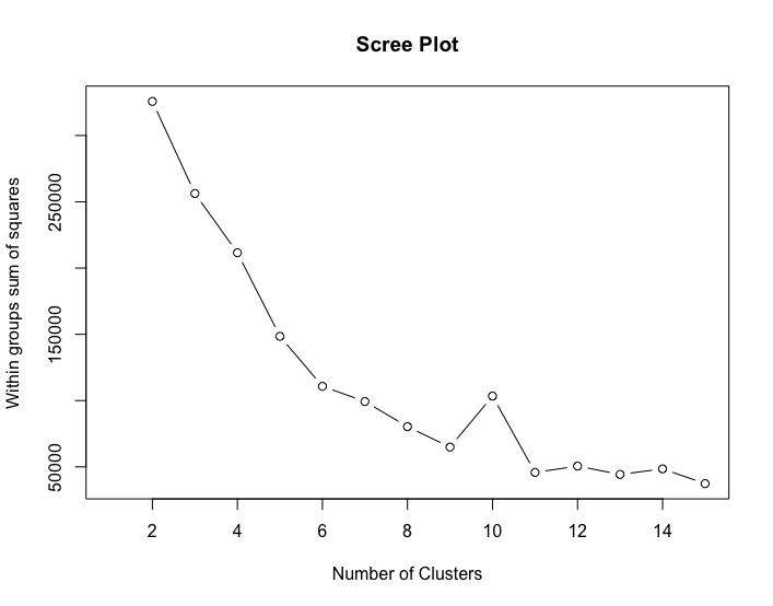
• Compute within-groups sum of squares (WSS) for k = 2 to 15.
• Plot to visually identify the “elbow” (around k = 10).

wssplot <- function(data, nc = 15) {
  wss <- rep(NA, length(2:nc))
  for (i in 2:nc) {
    wss[i] <- sum(kmeans(data, centers = i)$withinss)
  }
  plot(1:nc, wss, type = "b", xlab = "Number of Clusters",
       ylab = "Within groups sum of squares")
}
wssplot(matrix2)
title("Scree Plot")

Run K-Means Clustering:

• Fit k-means with 10 centers (chosen via elbow plot above).
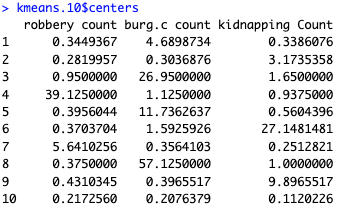
• Extract cluster assignments and centers.

set.seed(456)
kmeans.10 <- kmeans(matrix2, centers = 10)

Visualize Spatial Clusters:

• Assign colors using a qualitative palette (Paired + Set3).
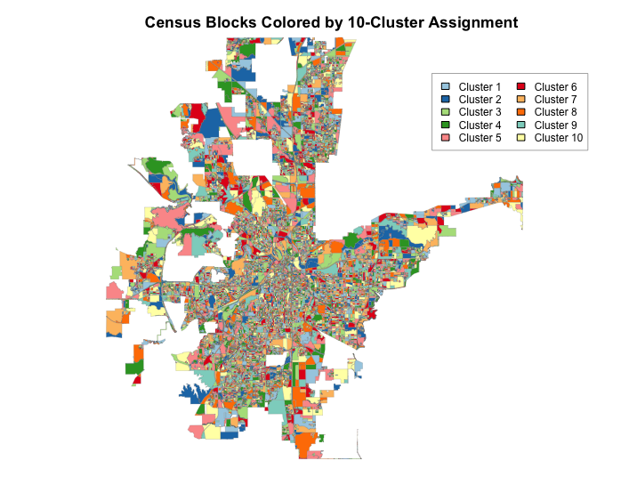
• Plot census blocks colored by cluster membership.
• Add title, legend, and thin borders for clarity.

cluster_colors <- c(brewer.pal(8, "Paired"), brewer.pal(3, "Set3")[1:2])
cols <- cluster_colors[kmeans.10map]   # kmeans.10map = kmeans.10$cluster (or sampled for demo)

plot(blocks, col = cols, border = "gray50", lwd = 0.2, main = NULL)
title("Census Blocks Colored by 10-Cluster Assignment", cex.main = 1.1, line = 2.5)
legend("topright", legend = paste("Cluster", 1:10), fill = cluster_colors,
       cex = 0.75, ncol = 2, bg = "white", box.col = "gray70", inset = 0.01)

Results and Interpretation:

• The elbow plot shows diminishing returns after ~10 clusters, selected k = 10 for balance between complexity and explanatory power.
• The final map reveals spatial groupings of blocks with similar combinations of robbery, commercial burglary, and kidnapping counts.
• Clusters may highlight:
  • High-robbery urban core areas
  • Commercial burglary hotspots (e.g., retail corridors)
  • Mixed or low-incident suburban blocks
• Further analysis could include cluster profiling (mean crime rates per cluster), spatial autocorrelation tests, or overlay with demographics.

Block groups per cluster

Mean counts of each crime type in each cluster